Instructions tested with Windows 10 64-bit.
It is highly recommend that you use Mac OS X or Linux for this course, these instructions are only for people who cannot run Mac OS X or Linux on their computer.
Table of Contents
Install and Setup
Spark provides APIs in Scala, Java, Python (PySpark) and R. We use PySpark and Jupyter, previously known as IPython Notebook, as the development environment. There are many articles online that talk about Jupyter and what a great tool it is, so we won’t introduce it in details here.
This Guide Assumes you already have Anaconda and Gnu On Windows installed. See https://mas-dse.github.io/startup/anaconda-windows-install/
1. Go to http://www.java.com and install Java 7+.
2. Get Spark pre-built package from the downloads page of the Spark project website.
3. Open PowerShell by pressing ⊞ Win-R, typing “powershell” in Run dialog box and clicking “OK”. Change your working directory to where you downloaded the Spark package.
4. Type the commands in red to uncompress the Spark download. Alternatively, you can use any other software of your preference to uncompress.
> tar xvf spark-2.1.0-bin-hadoop2.7.tar
5. Type the commands in red to move Spark to the c:\opt\spark\ directory.
> move spark-2.1.0-bin-hadoop2.7 C:\opt\spark\
6. Type the commands in red to download winutils.exe for Spark.
> curl -k -L -o winutils.exe https://github.com/steveloughran/winutils/blob/master/hadoop-2.6.0/bin/winutils.exe?raw=true
7. Create an environment variable with variable name = SPARK_HOME and variable value = C:/opt/spark. This link provides a good description of how to set environment variable in windows
8. Type the commands in red to create a temporary directory.
> cd ~/Documents/jupyter-temp/
9. Type the commands in red to install, configure and run Jupyter Notebook. Jupyter Notebook will launch using your default web browser.
> ipython kernelspec install-self
> jupyter notebook
First Spark Application
In our first Spark application, we will run a Monte Carlo experiment to find an estimate for $\pi$.
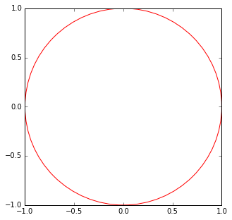
Here is how we are going to do it. The figure bellow shows a circle with radius $r = 1$ inscribed within a 2×2 square. The ratio between the area of the circle and the area of the square is $\frac{\pi}{4}$. If we sample enough points in the square, we will have approximately $\rho = \frac{\pi}{4}$ of these points that lie inside the circle. So we can estimate $\pi$ as $4 \rho$.
1. Create a new Notebook by selecting Python 2 from the New drop down list at the right of the page.
2. First we will create the Spark Context. Copy and paste the red text into the first cell then click the (run cell) button:
import sys
import findspark
findspark.init()
from pyspark import SparkContext
sc = SparkContext(master="local[4]")
3. Next, we draw a sufficient amount of points inside the square. Copy and paste the red text into the next cell then click the (run cell) button:
TOTAL = 1000000
dots = sc.parallelize([2.0 * np.random.random(2) - 1.0 for i in range(TOTAL)]).cache()
print("Number of random points:", dots.count())
stats = dots.stats()
print('Mean:', stats.mean())
print('stdev:', stats.stdev())
Output:
('Mean:', array([-0.0004401 , 0.00052725]))
('stdev:', array([ 0.57720696, 0.57773085]))
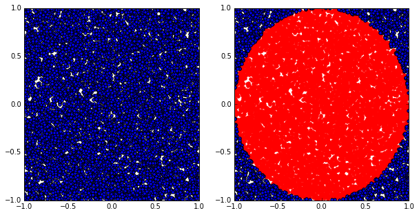
4. We can sample a small fraction of these points and visualize them. Copy and paste the red text into the next cell then click the (run cell) button:
from operator import itemgetter
from matplotlib import pyplot as plt
plt.figure(figsize = (10, 5))
# Plot 1
plt.subplot(1, 2, 1)
plt.xlim((-1.0, 1.0))
plt.ylim((-1.0, 1.0))
sample = dots.sample(False, 0.01)
X = sample.map(itemgetter(0)).collect()
Y = sample.map(itemgetter(1)).collect()
plt.scatter(X, Y)
# Plot 2
plt.subplot(1, 2, 2)
plt.xlim((-1.0, 1.0))
plt.ylim((-1.0, 1.0))
inCircle = lambda v: np.linalg.norm(v) <= 1.0
dotsIn = sample.filter(inCircle).cache()
dotsOut = sample.filter(lambda v: not inCircle(v)).cache()
# inside circle
Xin = dotsIn.map(itemgetter(0)).collect()
Yin = dotsIn.map(itemgetter(1)).collect()
plt.scatter(Xin, Yin, color = 'r')
# outside circle
Xout = dotsOut.map(itemgetter(0)).collect()
Yout = dotsOut.map(itemgetter(1)).collect()
plt.scatter(Xout, Yout)
Output:
5. Finally, let’s compute the estimated value of $\pi$. Copy and paste the red text into the next cell then click the (run cell) button:
print("The estimation of \pi is:", pi)
Output:
Next Steps
References
- Spark official documents
- Example Python Spark programs on the Spark Github repository